School of Agriculture and Natural Resources

An Introduction to ArcView® GIS

Developed By

Dr. Walid H. Shayya

Table of Contents

About GIS

A geographic information system (GIS) is a system of computer software, hardware, data, and personnel to help manipulate, analyze, and present information (visualization of data analysis) that is tied to a spatial (geographic) location.  In other words, GIS is a computerized data management system designed to store, manipulate, update, and output geographically- referenced spatial data.  In addition to producing basic maps (quickly, accurately, and update-to-date), GIS software nowadays are capable of performing basic to advanced analysis, varying from measuring distances, perimeters, and areas to dealing with proximity, connectivity, and containment as well as networking, buffering (flood zones, address notification), line of site (slope), and spatial analysis.  Thus, GIS is capable of numerous tasks including (but not limited) to the following:

• Input and update spatial and attribute (e.g., plot owner) data.
• Combine data from different sources.
• Link spatial data with attribute data.
• Analyze multiple data sets.
• Convert coordinate system.
• Convert data formats.
• Export to other data formats.
• Generate analog maps and tabular reports.

There are numerous benefits to using GIS.  These include, among other things, the following:

• Improved efficiency in dealing with geographically-referenced data.
• Better information for users and decision makers (graphical displays and spatial analysis).
• Greater consistency in information for users and decision makers.
• Improved interaction among individuals and organizations (technical elite versus public).
• Integrating research and education.

Geographic information systems are used by businesses, government agencies, and nonprofit organizations to describe and analyze the physical world.  Some of the numerous applications of GIS nowadays include the following:

• Emergency services (fire and police).
• Environmental monitoring and modeling.
• Business (site location and delivery systems).
• Government (local, county, state, federal, and military).
• Education (research, teaching, and administration).
• Agriculture (site-specific crop management and precision farming).
• Wherever spatial and geographical data analysis is needed.

About ArcView® GIS Version 3.x

ArcView is a useful software or desktop GIS and mapping.  It is a product of Environmental Systems Research Institute, Inc. (ESRI).  ArcView GIS is a powerful software that provides for visualizing, querying, exploring, and analyzing data geographically.  ArcView is a powerful GIS tool that can display information (which resides locally or over a distributed network), read spatial and tabular information from a variety of data formats, access external databases, produce thematic maps (use colors and symbols to represent features as well to represent features based on their attributes), perform spatial queries, connect spatial information to database attributes, provide several analytical tools, and allows for a high degree of customization using Avenue.  For further details, please refer to the ESRI website at http://www.esri.com.

Several versions of ArcView 3.x have been released to date.  This tutorial is very basic in nature and addresses general features of versions 3.0, 3.1, 3.2, and 3.3.  Although no distinction will be made in this tutorial amongst the four versions of ArcView, it is important to emphasize the added options and features that were included in each subsequent release of ArcView 3.x.  The following are some of the distinctive enhancements of the various releases of ArcView GIS over ArcView 3.0 (Sourse: ESRI White Paper):

• "ArcView 3.1 introduced a wizard-based approach to accomplish a variety of more sophisticated tasks such as advanced map production and advanced geoprocessing. Task wizards, along with other updates focusing on enhancing usability, leverage the power of ArcView to help you more quickly and easily accomplish your geographic information system (GIS) objectives. ArcView 3.1 also introduced several new included extensions, specifically designed to supplement your GIS requirements. In particular, ArcView features a report writer extension that enables you to easily generate professional reports, including embedded maps and charts, that help you more successfully communicate the results of your GIS analysis.
• ArcView 3.2 provided both strategic updates to existing capabilities as well as new tools to facilitate your GIS operations. Specifically, ArcView 3.2 included an updated report writer and significant database access improvements. ArcView 3.2 also introduced a new shapefile projection utility, providing support for an extensive range of data projections and datum transformations, as well as support for several new data formats.
• ArcView 3.3 provides key updates to many of the tools that are part of ArcView.  ArcView 3.3 includes updates to many extensions including CAD Reader, ERDAS IMAGINE® Image Reader, and the National Imagery Transmission Format (NITF) Data Reader. Also, the Projection Utility has been enhanced for greater performance. The Report Writer has been updated to include Crystal Reports™ 8.5 by Crystal Decisions. Database Access 2.1c is also included to support the latest ArcSDE™ database and provide direct connections to ArcSDE data. ESRI Data & Maps has also expanded to eight CDs full of new and updated data."

Several extensions are available for use with ArcView.  Many of these are commercial extensions developed by ESRI and others.  Some of the commercial extensions developed by ESRI include the following:

• Network Analyst: Performs network or routing analysis.
• Spatial Analyst: Performs grid cell (raster) analysis.
• Internet Map Server: A map publishing tool for the World Wide Web.
• StreetMap: A tool for U.S. Street address geocoding and map display.
• ArcPress: Develops maps on raster plotting devices.
• 3D Analyst: Creates, analyzes, and displays surface data.
• Business Analyst: Supports business analysis.
• Image Analysis: Supports image analysis capabilities.
• Tracking Analyst: Directs feed and playback of real-time data, including data from Global Positioning System (GPS).

Also, there are several free extensions available from ESRI:

• VPF Reader: Provides for reading Vector Product Format (VPF) data.
• Dialog Designer: Allows for creating and designing your own custom forms and dialogs with the ArcView GIS environment.
• MrSID Image Support: Supports multi-resolution wavelet-based image format.
• Database Access: Allows for accessing Spatial Database Engine (SDE) data.
• Military Data Reader Extensions: Allows for reading a variety of image data produced in the defense and intelligence communities.
• Database Themes: Supports SDE data.
• CAD Reader: Supports AutoCAD (DWG and DXF) and MicroStation (DGN) files.
• Digitizer: Supports digitizing and provides for directly entering your data using standard Windows WinTAB digitizer drivers.
• IMAGINE Reader: Supports reading and displaying ERDAS IMAGINE files.
• JPEG (JFIF) Image Support: Supports JPEG images for picture frames in layouts and for themes.
• GeoProcessing: Provides spatial analysis functions that include dissolve features, merge themes, clip, intersect, union, and spatial join.
• Crystal Reports:  External report writing program that runs under Windows.
• Graticules and Measured Grids: Provides for adding graticules and grids to layouts.
• Legend Tool: Provides for creating a customized graphical legend.
• TIFF Image Support: Supports reading TIFF images. 

Getting Started with ArcView® GIS Version 3.x

ArcView organizes the mapping project and the tools available to you within a system of windows, menu bars, button bars, and icons. The entire ArcView environment and GUI (grahpics user interface) are contained in the main application window.  When you first start ArcView GIS, you will see this window (a screen similar to the one depicted below).  

If you select the "as a blank project" option and click on the "Ok" button, you will see a window representing the project "Untitled".  A project comprises all of your work on a particular problem.  It may consist of many views (maps), tables, charts, page layouts, and Avenue programming language scripts.  Project file names have an ".apr" extension.  In order to give your project a more meaningful name than "Untitled", click the "File" option on the top menu bar, and select the "Save Project" option.  This will allow you to rename your project and store it on disk under any desired pathname.  Please note, however, that when you save a project, you are not saving the data but the pathnames to the data and the changes you have done to them.  This means that you will not be able to take the project to another computer, unless the data you work with are already available on that computer.  Otherwise, you need to copy the data as well before you can run your project on the other computer.  If the data are available on the other computer but is in a different subdirectory, you will need to help ArcView GIS find this data before the software can reconstruct your project.

Projects

A project is the highest organizational unit in ArcView.  An ArcView project allows the user to group all work components of a specific problem (views, themes, tables, charts, layouts, and scripts) into a single unit.  In other words, it is a collection of associated windows, or documents, that are displayed during an ArcView session.  The "Project" window contains all of the other documents associated with the project and are accessed through the active project window.  

Projects are text (ASCII) files stored with an ".apr" extension.  Project files contain pointers to the physical locations of the associated documents as well as user preferences (colors, GUI, window sizes, and positions).  The user preferences as stored within the project only affect the way the data is displayed (not the data itself).

When you create a new project (or open an existing one), a project window will appear in the ArcView window.  This lists all the components of the project and enables you to manage them. Double-click a component's name to open it.  The title bar of the project window shows you the name of the project.  When you open one of the components of a project, it is displayed inside its own window.  You can have any number of windows open in ArcView, but at any time there is only one active window.  The active window is the window you are currently working with.  All the windows that are currently open inside the ArcView window are listed at the bottom of the Window menu in the ArcView menu bar.  To make a window active, simply right-click inside it or on its title bar, or choose it from the list in the Window pull-down menu at the top of the ArcView window.  When you open a window it automatically becomes active.  If part of a window is hidden by others, making it active will bring it to the top.

Views and Themes

Views in ArcView can be thought of as maps.  Views are based on spatial data containing geographic locations of features on the earth's surface, along with attribute information describing what these features represent.  Each view has a "Table of Contents" that lists the themes in the view and shows what symbols and colors they are drawn with.  You also use the "Table of Contents" to control how the view is drawn.  To create a new (empty) view, click on the "New" button.  Like paper maps which are made up of lines showing roads, dots showing cities, and areas showing states, a view can be made up of several "themes".  Each theme shows one type of feature on the map.

Types of Themes

There are two broad types of themes.  These include raster or grid (pixels or picture elements) and vector themes (points, lines, and polygons).  Aerial and satellite photographs can be displayed as "image" or "raster" themes in ArcView GIS.  Though the ability to display images is very important in many applications, it is difficult to store additional information about objects seen in the images.  This is because the image is not made up of objects, but rather of the individual pixels that constitute the photograph.

Vector themes, on the other hand, represent specific features in the real world.  Additional information about each feature (referred to as feature attributes) are stored in a linked "attributes" table.  In general, there are three types of vector themes: point, line or arc, and polygon.

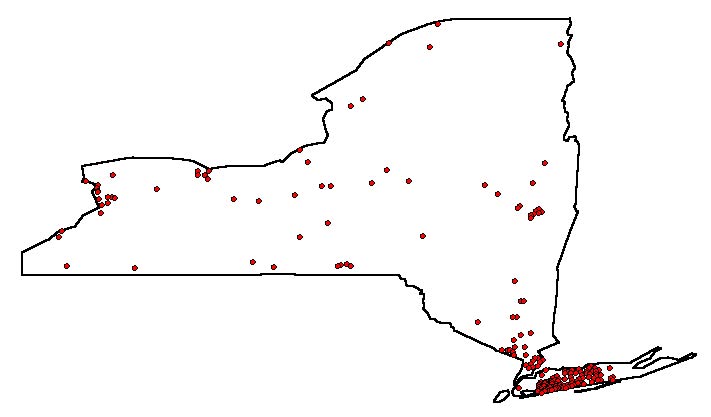
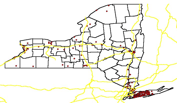
Point themes show where things are.  Point themes can be used to indicate the locations of buildings, trees, sampling sites, and other objects (such as cities) which are relatively small in relation to the area covered by the map.  Each dot in the figure below shows a city in the State of New York.  Points have location but no extent (zero dimension).  You could modify the map so that bigger cities in population have bigger dots.  However, the relative size of each city is not truly indicated by the map.  

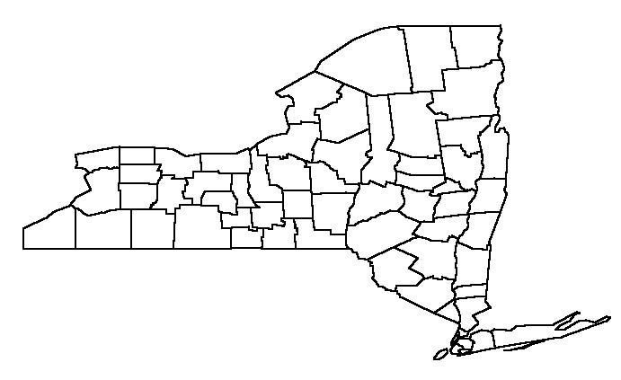
Polygon themes are used to represent features that have area (such as countries, states, national parks, city blocks, school districts, and watersheds).  The theme shown below depicts the counties within the State of New York.  In this theme, each county is a separate entity stored along with its corresponding attribute information such as area, population, number of farms, and demographics.

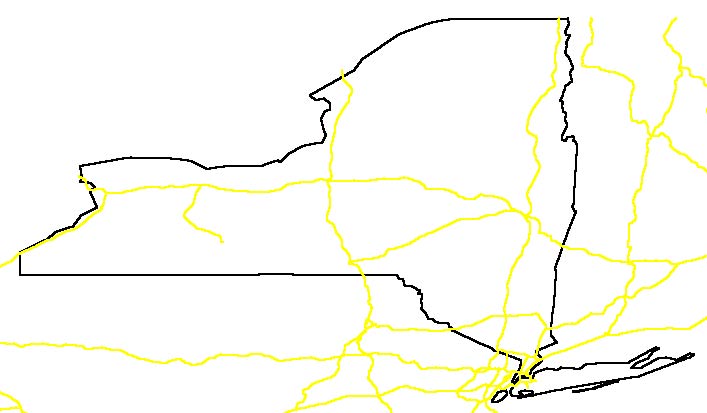
With few exceptions, general vector themes can only be of one type.  A theme is either a point, arc or line, or polygon.  However, one may combine several themes of various types into one view.  This enables the individual to look at different factors in relation to one another. For example, one could combine the boundaries of counties (polygon theme), cities (point theme), highways (line theme), and boundaries of the State of New York (polygon theme) to produce a view similar to the one shown in the figure below.  With this View, for example, you might be able to identify the interstate highways within the State of New York that provide the best routes among major cities within the State.

Tables

Tables are ArcView’'s representation of data. They contain descriptive information about specific subjects.  Each row (or record) defines one entry in the database (e.g., one county polygon) while each column (or field) defines a single characteristic for the entry (county name).  Any database file (dbf, INFO, or ASCII) can be displayed as an ArcView Table.  Regardless of the source of table, all tables appear the same to the user in ArcView.  ArcView defines a standard template to reference the table the user accesses.  The tabular data itself is not imported, but rather continues to be stored in the source file in its native format. The ArcView link to the data is dynamic (i.e., changes in the data outside ArcView will be reflected in ArcView projects that reference these data).

Charts

Charts in ArcView GIS are very useful tools to display, compare, and query data.  Charts provide graphic representation of summarized tabular data (especially attributes of geographic features) that can quickly convey information.  Charts can also query geographical and tabular data.  Charts in ArcView are especially powerful since they are linked to the themes in a view.  A chart is dynamic so it reflects the current status of the data in the table. If you edit the table in ArcView, the chart will immediately reflect the edit.  If the tabular data source is edited, the change will be reflected in the table and the chart when you choose "Refresh" button from the "Table" menu or the next time you open the project.

Different charts representing your data can be created for different purposes.  Six different chart types are available in ArcView: line, bar, column, xy scatter, area, and pie.  Each contains a variety of chart styles for you to choose from.

Scripts

Script windows are for writing and displaying Avenue scripts that customize the ArcView user interface or perform predefined tasks.  Avenue is ArcView'’s object-oriented programming language. With Avenue you can modify the appearance of ArcView, create new programs, make complex tasks simple, and communicate with other applications such as ArcInfo, relational database managers, and spreadsheets.  Although scripts provide very powerful customization tools in ArcView GIS, they are beyond the scope of this introductory tutorial and, therefore, will not be covered.

Making Simple Thematic Maps Using ArcView® GIS Version 3.x

A thematic map is one that shows something about a geographic area besides location.  Our focus in this section is to develop two simple thematic maps.  One of these maps will show the distribution of population in the counties of the State of New York while the other will display the change in population in these counties between 1990 and 1999.  As we develop these simple maps, we will review along the way the various basic components of ArcView GIS.  

Adding Themes to a View

We begin by creating a view by clicking on the "New" button to create a new, empty view.  You could also create a new view by double-clicking on the "Views" icon in the project menu.  Either option opens up a new view for you to work with.

Adding themes to the view can be accomplished by either clicking on the button or clicking on the "View" in the upper menu bar and selecting the "Add Theme..." option from the pull-down menu.  Either of these options will open up a navigation tool, similar to the one depicted in the figure below, to enable you to select the theme you want to open.

You will notice the selection space labeled "Data Source Types:" where two options are available.  These include the "Feature Data Source" option that includes the point, line, and polygon themes discussed above as well as the "Image Data Source" option that provides for including raster themes (such as aerial and satellite photographs).  Our intention in this introductory tutorial is to use vector data based on points, lines, and polygons.  For this reason, we will leave the default selection for data source (i.e., "Feature Data Source").

To start our exercise, let us use the data provided with ArcView.  The pathname depicted in the figure above represents the default location of data files provided with ArcView.  Since we are interested in working with New York State Data, let us double-click on the subdirectory named "usa" that contains data for the USA. 

A theme (vector in this case) can then be selected by clicking on the name of the desired shape file (file with extension "shp") from the list of files followed by clicking on the "Ok" button (or you may double-click the file name to accomplish the same task).  If we select the "Counties.shp" file from the list of available themes in the "usa" subdirectory, the name of this theme is displayed in the table of contents of the view, to the left of the view window as depicted in the following screen.

However, the theme itself does not display until you click within the checkbox to the left of the theme name.  Here is a display of the theme that shows all of the counties of the United States.

You may repeat the procedure described above to add one or more themes to your view.  

Moving Around in a View

You can move around and change the display in a view using several available tools.  These tools are available in the tool bar described in the following screen.  The best way to learn these tools is to try them out.

Redefining a Theme

The theme representing the counties of the United States of America was displayed earlier.  Since the focus of our exercise is to work with the counties of the State of New York, let us redefine our theme.  The properties of any theme can be viewed by first making the theme active (by clicking on the theme title in the table of contents of the view).  This is different than checking the title of the theme which will prompt ArcView to display the theme in the given view.  Once the desired theme is active, clicking the "Theme" tool on the top bar will show a pull-down menu.  By clicking on the first option of this menu (i.e., "Properties..."), a screen similar to the one presented here will appear.

Through this dialog box, you can change the name of the theme, set rules for labeling features, set rules for editing features, set rules for geocoding, and decide at which scale a theme will display.  We can redefine the theme to include only the counties in the State of New York.  This can be accomplished by first clicking on the "Definition" icon (if not already highlighted) and then clicking the "Query Builder" icon .  This opens up the following "Query Builder" dialog box.

Since we are dealing with a geographic information system, each feature has several attributes in addition to the geographic ones showing the outline of a county.  In this case, we have information regarding each county (attributes) in a form of a number of fields (Shape, Name, State_name, etc...).  The "Query Builder" dialog box lists the fields, a group of allowable operators, and the available values for a field (once a field is selected as shown in the screen below).

Since one would expect the state name of each county in the union to be listed in the "State_name" field, we assume that all New York counties will have the word "New York" in the "State_name" field and that this would be a good way of sorting out those counties.  To accomplish this, we may build a definition for our theme so that it includes all counties for which State_name="New York" as depicted in the following screen.

More complex queries are also possible, using the available Boolean and mathematical operators. For example, we can use the following queries:

• ([State_name]="New York") or ([State_name]="Ohio"):  This definition eliminates all entries except those that have "New York" or "Ohio" in the "State_name" field.
• ([Area]>400):  This definition eliminates all entries except those that have a value exceeding 400 in the "Area" field.
• ([State_name]="New York") and ([Area]>400):  This definition eliminates all entries except those that have "New York" in the "State_name" field and a value exceeding 400 in the "Area" field.

After you click "OK" on the Query Builder dialog box, and click "OK" again on the "Theme Properties" dialog box, you eliminate all the counties except those in the State of New York.  After you click on the "Zoom to Full Extent of View" button, you are left with a display of the State of New York which fills the window.

The attributes of any feature in the "active" theme can be viewed by first selecting the Identify tool (), and then clicking on the feature (such as Madison County, New York) that you may want to identify (see sample screen below).

Remember that themes are drawn in the bottom-to-top order in which they appear in the table of contents bar to the left of the view window.  If a theme is covered over by another theme, you can make it visible by clicking and dragging its symbol upward in the table of contents.

Projections

By default, "views" have no specified projection in ArcView.  Data in ArcView 3.x are assumed to be in decimal degrees of latitude and longitude, without taking into account the fact that degrees of longitude get smaller the further north of the Equator you go.  ArcView 3.x, however, provides the utility for projecting shapefiles, grids, and images in any projection or reference system.  If the themes in a view are all latitude-longitude data, you can specify a projection for your view and ArcView will re-draw the map in that projection.  The projection utility supports a number of projections and datum conversions (including NAD27 to NAD83) as well as customization of projections.  Additional themes such as grids or images which are based on the selected projection can also be added.  However, one must remember that a view cannot reconcile themes in different projections.

To display the projection of the current active view, click on the "View" option in the top menu bar and select the "Properties" option from the pull-down menu.  A "View Properties" dialog box, similar to the one displayed below, will be displayed..

The "View Properties" dialog box allows for setting the properties of "View" parameters (including map and distance units that provide for measuring distances in the view and creating an accurate scale bar for the final map).  To change a projection, you need to double-click on the "Projection" button to bring up the "Projection Properties" dialog box that allows you to alter the projection of the view.  When you specify a view projection in the "View Properties" dialog box, ArcView will display shapefiles with latitude-longitude decimal degree coordinates in the specified projection.  If all the shapefiles in a project are in latitude-longitude decimal degrees, a view projection can make the map look a lot better.  Un-projected latitude-longitude maps of large areas can look very distorted.  

Working with Theme Attributes

After completing the previous section, it is obvious that all counties in the resultant map of the State of New York are displayed in one color.  To start out, let's make a map that shows something simple, such as the distribution of population within state counties.  You should keep in mind that the map developed so far is a geographic information system where tabular information are linked to each feature in the map representing the state counties.  To see all the available information for each of the counties, click on the Open Table tool ().  This opens up the basic table for the active theme table (or theme attributes) as shown below.

This particular table includes a list of all the field we have seen earlier while defining theme properties.  Such fields include Shape (polygon), Name (county name), State_name (New York), State_fips (State Federal Information Processing Standard), County_fips (County Federal Information Processing Standard), Fips (Federal Information Processing Standard combining the State and County FIPS), Area, Pop1990 (county population in 1990), Pop1999 (county population in 1999), and numerous other fields.  The FIPS code will be helpful when joining tables, since there is a unique FIPS code to identify each county in the United States (although many different states may have similar county names such as "Lincoln" and "Washington" counties).

To make a map based on population, we need to go back to the View. The easiest way to do this is to click on the "Window" option in the top menu bar, and select the view (View1 in this case).  Underneath the name of the theme (currently "Counties.shp") in the table of contents of the view are a number of boxes, each representing a state.  These entries are still displayed based on the original theme data which is no longer displayed since we have selectively chosen to only display the counties of the State of New York.  To change this, double click on any of the boxes to display the Legend Editor as shown below.

The "Legend Editor" allows you to change how features in a theme are displayed, either as a whole, or according to the values in a specific column of the table.  Since "Counties.shp" is a polygon theme and the "Legend Type:" was selected as "Unique Value" (with the "State_name" field representing the "Values Field:"), colored box symbols appear in the "Legend Editor" for each of the 50 states in the union.  If you were working with a "Single Symbol" "Legend Type:", you may change the color or style of the symbol for all features in the theme by first pointing to the symbol and then double-clicking (the symbol will be a colored rectangle for a polygon theme, a colored line for a line theme, a dot or other point symbol for a point theme). ArcView will display a palette from which you can choose colors, styles, border widths, and other display parameters. When you click on "Apply," the changes are applied to the map.  

The color of all counties in the State of New York is the same.  To make the fill-in colors of the county features appear differently based on their 1999 population, we need to first select the "Graduated Color" option for "Legend Type".  The first field in the theme attributes table will be the default "Classification Field".  Since we intend to have a map that shows the distribution of population among counties based on 1999 data, we ought to choose the "Pop1999" field.  This prompts ArcView to produce a colorful thematic map in which each color indicates a difference in value as depicted in the following screen.  

Underneath the "Classification Field:" selection box is a box labeled "Normalize by:".  This allows you to divide the values in the selected classification field by the values in the field specified in the "Normalize by:" box.  In this case, you may specify the "Area" field, and get a map based on population density.

By default, ArcView breaks up the features into five groups, based on the "Natural Breaks" statistical method.  You can change the number of categories and the type of statistical classification by clicking on the "Classify..." button.  You can choose one of the following classifications: "Equal Area", "Equal Interval", "Natural Breaks", "Quantile", and "Standard Deviation".

Opening up the "Color Ramps:" menu bar lets you choose a different set of colors than the default "Red monochromatic" ramp colors. If none of the available color ramps are suitable, you can change each color individually by double-clicking on the corresponding symbol.  This will bring up a color and style palette.

Of particular significance in some situations is the button marked with a zero ().  This button lets you specify how to display null or dummy values as well as avoid using these numbers in statistical calculations.  In many instances, cells for which data are not available are marked with a specific dummy value (e.g., "-99").

You may also want to round off numbers and change the way that each grouping is labeled in the map legend.  To do this, click in the "Value" cell that corresponds to the group that you wish to change and type in the values that you want included (e.g., you could change the lowest value for the first group from "5180-166219" to "5000-150000," and alter the next group accordingly.  The "Label" fields will automatically change to match, but you can also change them manually to something like "Low", "Low-Medium", "Medium", "Medium-High", and "High" (if you so desire).

For the sake of this exercise, we will accept all the defaults by clicking the "Apply" button without making any further changes.  This results in the following view.

Working with Tables

The "attributes of Counties.shp" that we have worked with so far includes an extensive list of information for each county.  We could, however, expand this table by adding more columns to the table, or even joining several tables together.  We can also create our own tables, either in ArcView or using other software including spreadsheet or database programs.

To add a table to the project, return to the "Project" window, click on the "Tables" icon, and then click the "Add" button.  This enables you to navigate to the directory where you can find the desired table in "dbf" format.  The figure displayed below shows some of the available database files that are supplied with ArcView.  You will realize that these files correspond to a similar list that appeared earlier while displaying the themes provided with ArcView shape files, including the one used in this workshop (i.e., "Counties.shp").  The "states.dbf" file was selected in the figure below only for the sake of demonstration.

Tables can also be linked after finding one column in each table that contains a unique identifier by which the linking can occur.  For example, we could use the two-digit State_fips number to join the two currently loaded tables (i.e., "Attributes of Counties.shp" and "states.dbf").  The "State_fips" field uniquely identifies each state and appears in both tables (FIPS codes are also assigned to smaller geographic units, down to the level of Census blocks).  To join these two tables for example, we highlight the common column header in each table and click on the "Join" button () which becomes active only after a column header in each of the two tables is selected (data format in the column must be the same).  The active table at the time the "Join" button is pressed will have the combined data (although data won't be transferred among tables but rather the details of the operation are maintained by ArcView).

Adding a column to a table using ArcView can be accomplished either by keying in your own data or having ArcView calculate the values in the new field (column) based on the data in other fields (columns).  To append a field to a table, click on the "Table" option from the menu bar (appears when the attribute table is active), and select the "Start Editing" option from the pull-down menu.  Then click on the "Edit" option in the menu bar and select the "Add Field..." option.  This opens up the "Field Definition" dialog box as shown below.

The "Field Definition" dialog box allows the user to give the new field a name, decide whether the new field is a number or a string (alphanumeric) field, and specify the number characters (including decimal places) the field will contain.

To demonstrate this concept, a field will be added to the attributes of "Counties.shp" table representing the percentage change in population in the counties of the State of New York between 1990 and 1999.  Accordingly, the field name "PopChange" will be entered in the "Field Definition" dialog box to represent this field while the remaining default entries are retained as depicted in the following screen.

After making these changes and clicking the "OK" button, a new empty field will be appended to the table as shown below.

To have ArcView calculate the values in the new field, click on the "Field" option in the top menu bar and select the "Calculate..." option from the displayed pull-down menu.  After you select the new field (here named "PopChange), the "Field Calculator" dialog box will help you create the formula based upon which the values in the new field are to be calculated.  Here we will take the difference between the 1999 and 1990 populations to obtain the change in population (positive for an increase and negative for a decrease in population) as depicted below.

When the counties theme is displayed with the properties defined based on the added field, a map similar to the one displayed below results.

Labeling Features in Views

In many instances, you may want to label each feature in a theme with a name and/or some other field from the "attributes" table.  ArcView makes it easy to create labels but the final placement of labels can be time consuming.  In some instances, experimenting with several different fonts and type sizes may be necessary when working with small maps.

There are two different ways to label features.  The "Label" tool () allows you to click on a feature and to only label that feature.  Clicking on "Theme" in the menu bar and selecting "Auto-Label" will prompt ArcView to label all of the features in the active theme. The field from which the label is taken, and its placement relative to the feature is set through the "Theme Properties" dialog box.

Auto-labeling, in particular, may require some additional work.  If we were to label all counties in the State of New York for example, many of the labels would overlap several counties, while some labels may overlap each other.  Some of these problems can be avoided through the auto-label dialog box.  This box appears when you select the "Auto-label..." option from the pull-down menu that appears after selecting the "Theme" option from the top menu bar.

Sometimes, it may be helpful to change the type font, size, and style.  This may be accomplished by clicking on the "Edit" option in the top menu bar and selecting the "Select All Graphics" option from the pull-down menu  (labels are considered graphics, so they will all be selected).  Then call up the font menu (by clicking on the "Window" option in the top menu bar) and select the "Show Symbol Window..." option from the pull-down menu as shown below.

Clicking on the "ABC" icon will bring up the font palette through which you can change the font, size, and style of labels.  To change the location of any label, you just need to select the "Pointer" tool () and click on a label and drag it to the proper place.

Adding One's Own Features

Already existing points, lines, and polygon features may not be all what you need to use as you may want to add your own features.  To do so, click on the "View" option in the top menu bar and select the "New Theme..." option from the displayed pull-down menu.  This brings up a dialog box from which you can specify whether you want to create a point, line, or polygon theme as depicted in the following screen.

Selecting one kind of theme brings up the dialog box where you can give the new theme a name and specify where it will be stored.  

Once a new name is selected and the "Ok" button is pressed, the right set of options from the drawing tool are displayed.  For example, if you were to create a polygon theme, you may choose to select a feature among a number of ones (including rectangular, round, or free-form polygons as shown below).

When you draw a point, line, or polygon, you automatically create a blank row in a table. The cell for the feature you draw indicates whether it is a point, line, or polygon. You can you tell which line in the attributes table corresponds to which feature using the "Selection" tool.  First, you will need to select a row in the attribute table, resulting in the corresponding feature being also selected.  If you select a feature, the corresponding line in the attributes table is also selected.

Layouts

Layouts are used to combine all other documents (views, tables, and charts) into an output document (usually a hardcopy map).  Any previously composed view can be placed into a layout.

Once you develop a view that reflects the basis of a desired graphical output, your next step is to put this view into a map layout.  A layout includes the view you've created, a scale bar, a North arrow, other graphics, and a legend table that explains the meaning of various symbols in the view.

To create a layout, click on the "View" option in the top menu bar, and select the "Layout..." option from the pull-down menu.  A "Template Manager" window will provide you with several existing standard map formats.  For example, you may choose between landscape and portrait paper orientations and decide whether or not to include neatlines in your map.  After you make your selection, ArcView will create a layout for you (see sample below).  Items in this layout can be resized, moved, or deleted.

Alternatively, you may return to the "Project" window, and double-click on the "Layouts" icon. This will create a blank layout sheet and activate the "View Frame" tool.  With this tool, you can place the View, legend, scale bar, and North arrow anywhere you like on the page.

The layout you create can be printed or exported as a graphics file in several formats (such as Bitmap, Windows Metafile, CGM, or Adobe Illustrator file).  To do so, select "File" from the menu bar, and choose "Print" or "Export" from the pull-down menu.

Concluding Remarks

Before you end your ArcView session, you should save your project if you intend to continue working on it in the future or want to save a copy for future reference.  To do so, click on the "File" option from the top menu bar and select the "Save Project" option from the pull-down menu.  The next time you begin working on this project (or any other project), choose the "File" option from the top menu bar and select the "Open Project..." option from the pull-down menu. To end your ArcView session, choose the "Exit" option from the same pull-down menu.

I hope that you find this introductory tutorial to ArcView GIS informative and useful.  As you can see, there are many more buttons and tools that were not demonstrated in this tutorial.  You can see their functions by just trying them, or can click on the "Help" option on the top menu bar and get help.  The help screen provide a good overview of the software.